

This page includes alternative methods for ultrasound data analysis. It includes information on Principal Component Analysis (PCA), done in MATLAB, and Temporally Resolved Articulatory Configuration Tracking of UltraSound (TRACTUS).
Principal Component Analysis (PCA)
This is a method that is separate but potentially complementary to contour analysis, described on Preparing and Analyzing Ultrasound and Video Data. This section includes the following information:
- PCA-based Analysis on the NCSU Phon Server
- PCA-based Analysis on any computer using TRACTUS
PCA-based analysis on the phon server
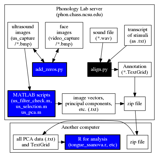
To do a PCA analysis of your images, follow these steps. For this example we will assume you have ultrasound images with the following location and name:
/phon/myproject/us_capture/mydata_000001_1.bmp
Change “myproject” and “mydata” as needed. Log in to the server to get started. Chances are you have a us_capture directory full of images from your recording, and some of the images were generated before or after your speaker was speaking, or they are during pauses. You can exclude these images from your analysis using a TextGrid file like this:
/phon/praat/praat /phon/scripts/skip_gaps.praat /phon/myproject/mydata.TextGrid 2 2 /phon/myproject/us_capture/
mkdir /phon/myproject/pca
cp mydata_filelist.txt /phon/myproject/pca/
cp mydata_misc.txt /phon/myproject/pca/
This will run the Praat script skip_gaps.praat, which reads your textgrid and the contents of your us_capture directory. If you do not have textgrid annotations indicating the locations of occlusal plane and palate images, only run the first copy command which makes a list of all the files, and indicates whether they should be included in the analysis. The first 2 in the call to the script tells it that a gap is any silence longer than 2 seconds. The second 2 tells the script that the word tier is tier 2 in your textgrid. If you have occlusal plane and palate textgrid annotations, the first column of ones and zeros in “mydata_misc.txt” corresponds to the occlusal plane and the second column corresponds to the palate. After skip_gaps.praat runs (which may take a few minutes), make a pca directory in your “myproject” directory, and copy the file list into it, so the Matlab scripts will find it.
Type this to enable MATLAB for this session:
add matlab81
The MATLAB functions will filter all of your images to enhance the tongue contour. The first step is to try two different filter settings and choose the best one. Enter this command to make the sample filtered images.
matlab -nodisplay -nosplash -nodesktop -r "P=path;path(P,'/phon/PCA');us_filter_check('mydata','bmp','/phon/myproject/us_capture/','/phon/myproject/pca/');exit"
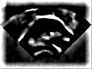
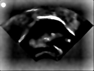
This will produce mydata_LoG_1.jpg and mydata_LoG_2.jpg in /phon/myproject/pca/ Download them and look at them, and decide which does the best job of enhancing the tongue surface without enhancing too much else. For example, see the sample filtered images below where the second (right-hand) image is preferable.
Next, enter this command to make a composite image from a sample of all your images. If you liked mydata_LoG_1.jpg the most, enter it with the 1 after ‘bmp’. If you liked mydata_LoG_2.jpg the most, put a 2 there instead.
matlab -nodisplay -nosplash -nodesktop -r "P=path;path(P,'/phon/PCA');us_selection('mydata','bmp',1,'/phon/myproject/us_capture/','/phon/myproject/pca/');exit"
This will produce a file called test_selection.jpg that is an average of a sample of your images, so that you can determine the range of the tongues movements, and define a region of interest to restrict your analysis (so you don’t waste time calculating the values of pixels where the tongue never goes). To define the region of interest, copy the file to the /phon/upload/ folder:
cp /phon/myproject/pca/mydata_selection.jpg /phon/upload/test_selection.jpg
Then go to the image mask page in a web browser. Enter “test_selection.jpg” in the “Image” field, and click Submit. You may need to refresh the page before the correct image appears. The image will appear with a blue overlay (the mask), and the points that appear at the bottom of the page define the polygonal window in the mask (the region of interest). Copy the numbers into the “Polygon” field, make a change, and click “Submit” to see the result. You will have to keep pasting them back into the field to change them. The letters “NW”, etc. are just there to help orient you, and you can use more or fewer points than the default of eight. When you have adjusted the points so that you can see the tongue through the window and the blue mask only covers the places the tongue doesn’t go, click the “Make mask from this polygon” checkbox and click submit one more time. Now there should be a .csv file in the /phon/upload directory. This file will tell the next script which pixels to keep in each image. Copy it to your folder:
cp /phon/upload/test_selection_mask.csv /phon/myproject/pca/mydata_mask.csv
Finally, run the PCA analysis, using the filter setting and image mask you chose. The 1 after ‘bmp’ is still the filter, so use 2 if you preferred 2. The next argument is the image downsampling factor (0.3, in the example below). This number determines how much the image resolution will be reduced. For this argument, use a value between 0 (no resolution) and 1 (full resolution). The fifth argument is the counter-clockwise angle of occlusal plane rotation (15, in the example below); use this argument to rotate images to the speaker’s occlusal plane. The sixth argument is the PC number or threshold (20, in the example below). If an integer value is used, the PCA function will retain that many PCs in the output. If, however, a non-integer value between 0 and 1 is used, the PCA function will interpret this number as a percentage threshold. In this case, the PCA function will retain as many PCs as are required to explain the given percentage of variance. For example, if you put 0.8 as a value for this argument, the output will retain as many PCs as are needed to explain at least 80% of the total variance in the image set.
We can process about 10 frames per second (but we record at 60 frames per second), so processing takes about six times real time. That means a 10-minute recording will take about an hour to process. For this reason we will run MATLAB using the command “nohup”, so that the process will keep running even if you lose your connection to the server. First we need to create a file to contain the commands we want to send to MATLAB. Enter this, replacing everything (mydata, myproject, 1) as you normally would:
echo "P=path;path(P,'/phon/PCA');us_pca('mydata','bmp',1,0.3,15,20,'/phon/myproject/us_capture/','/phon/myproject/pca/');exit" > /phon/myproject/pca/pca_cmd
If you need to redo the last step, you can edit the file /phon/myproject/pca/pca_cmd as you would edit any other file, or you can use “rm” to delete it and run the “echo” command again.
Now feed these commands to MATLAB:
nohup matlab -nodisplay -nosplash -nodesktop < /phon/myproject/pca/pca_cmd &
You can press enter several times to get back to the command prompt, and if you are still logged in when the script finishes, you will see a “Done” message announcing that.
Six new files will have been created in /phon/myproject/pca/. The first three are the most immediately useful, but you may want the other three later.
- mydata_pc_data.txt contains PC scores. Columns are PCs and rows are observations.
- mydata_filenames.txt contains the names of the images files, in processing order.
- mydata_pca_heatmaps.txt contains the loadings of the PCs in an n-by-m array
- Rows = y-coordinates of PC loadings
- Column 1 = PC number for corresponding row
- Columns 2-m = x-coordinates of PC loadings
- mydata_res_heatmaps.txt contains the residuals of the PCs in an n-by-m array
- Rows = y-coordinates of PC residuals
- Column 1 = PC number for corresponding row
- Columns 2-m = x-coordinates of PC residuals
- mydata_pca_output.mat is an n-by-m cell array for x PCs.
- Rows are n observations, and columns are:
- 1: filename
- 2: PC1 score for the file associated with row n
- …
- m-1: PCx score for the file associated with row n
- m: cell containing cumulative percentages of variance explained by PCs
- NB:
- cell {2,m} contains the discretation factor used in the analysis
- cell {3,m} contains the speaker name declared as an INPUT argument
- cell {4,m} contains the LoG filter parameter set used
- cell {5,m} contains the number of PCs retained
- cell {6,m} contains the the PCA variance threshold (if used)
- mydata_vecs.bmp is a bitmap image which contains the matrix that served as the input to the PCA.
To get started, download mydata_pc_data.txt, mydata_filenames.txt, and
mydata_pca_heatmaps.txt. If you are in ENG584 and you got to this point, check out these scripts for working with contours: tongue_trajectories.r (functions), tongue_ssanova.r (supersedes earlier SSANOVA functions), formant_functions.r (slighly updated), and plot_contours.r (commands to paste in, analogous to get_many_formants.r), and you can also ask one of your instructors.
PCA-Based Analysis using TRACTUS and MATLAB
TRACTUS (Temporally Resolved Articulatory Configuration Tracking of UltraSound) is a suite of GUI-based functions which perform PCA-based ultrasound analysis; it is intended for public use on computers which have MATLAB licensing but do not have access to the functions on the NCSU Phonology Lab server. This can be done on any computer wit ha MATLAB license. It is designed to perform temporal analysis on ultrasound images without the need for tracing of tongue contours. The analysis is based on a principal component analysis (PCA) model which includes ultrasound frames as observations and pixel intensity values as dimensions. Through orthogonal transformation of the data, the PCA model identifies linearly uncorrelated variables (principal components, PCs) which account for the greatest amount of variance in the data. TRACTUS generates PC scores for each ultrasound frame, and orients PC loadings (i.e. correlation coefficients) onto their original spatial location, which are saved to the user-specified results directory as heatmaps which allow the user to visually examine the articulatory configurations associated with each PC. The PC scores which are saved to the results directory can be plotted and analyzed as temporal vectors which determine the extent to which each ultrasound frame is correlated with the given PC and associated heatmap. These scores and loadings can also be transformed via linear discriminant analysis, linear correlation, etc., with classes/priors based on any number of relevant categories (e.g., consonant place of articulation, front diagonal of the vowel space, etc.) in order to generate a temporal vector which is associated no longer with an individual PC, but with how the PCs are correlated with phonetically/phonologically relevant groups.
An example of the output from TRACTUS is demonstrated in the images below for production of the word “ban”, with PC scores transformed through linear regression to approximate the acoustic diagonal of the front of the vowel space (i.e. Z2-Z1). This transformation results in a signal which corresponds to fronting/raising along an “articulatory diagonal”, i.e. lingual tensing. Clockwise from the top left, these images show: 1) the raw ultrasound frames, 2) the spectrogram and articulatory tensing signal, 3) PC loading heatmap associated with the transformed data, 4) composite frames generated from the cumulative weightings of the first 20 PCs; these frames approximate the original raw ultrasound image, but are generated solely from the first 20 PCs determined by the PCA model. They have also been rotated counter-clockwise to be parallel to the occlusal plane.
How to obtain TRACTUS
The following pages provide step-by-step instructions on how to download and use the TRACTUS functions, as well as how to interpret the results.
DOWNLOADING FILES
The files associated with TRACTUS are available at the following address:
http://phon.chass.ncsu.edu/tractus/
There are two primary functions which must be downloaded, ‘TRACTUS_prep.m‘ and ‘TRACTUS.m‘. Addtionally, all of the required functions must be downloaded separately. TRACTUS will need these functions in order to run properly.
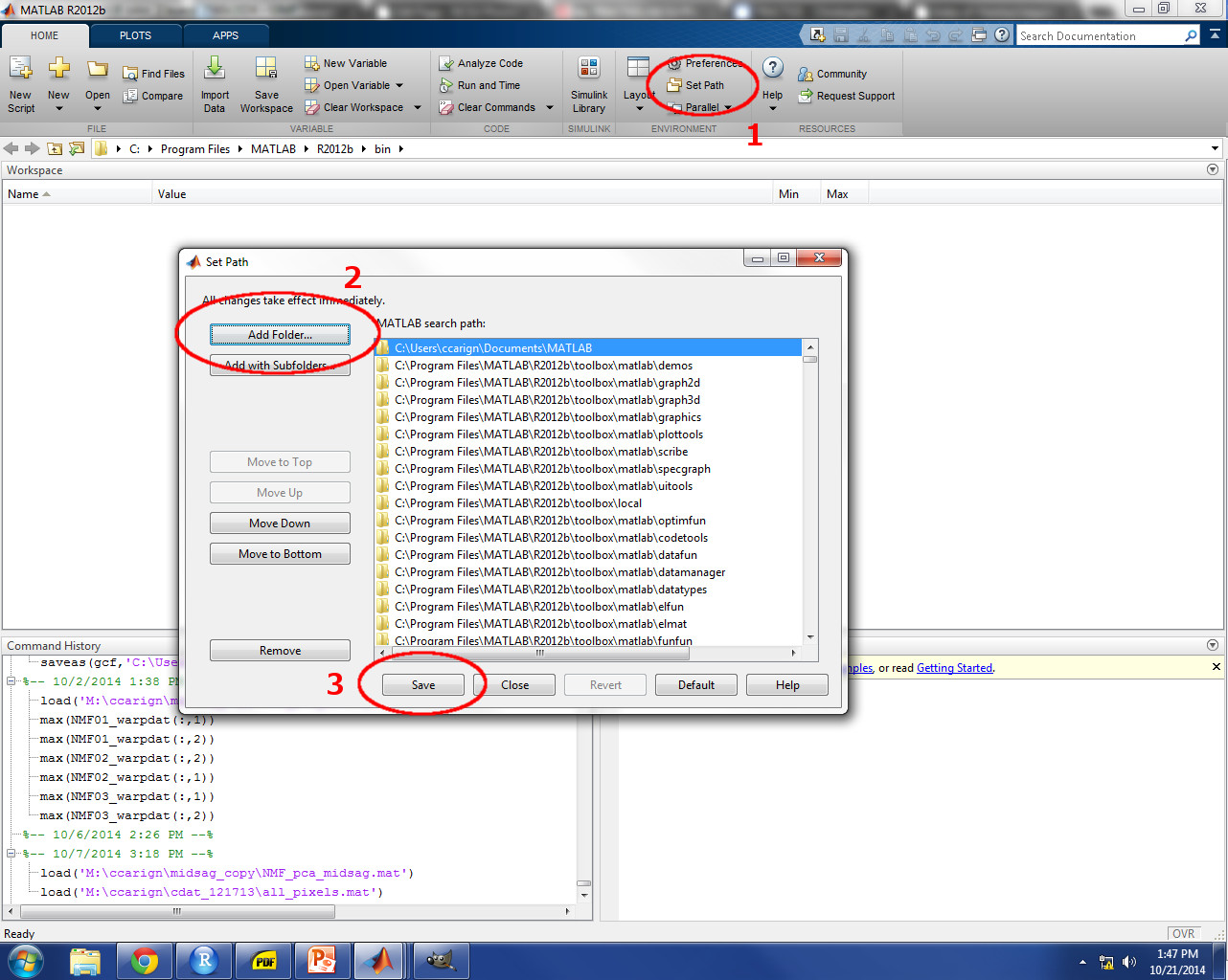
In order to use TRACTUS, you must first obtain licensing for the MATLAB software and its toolboxes. Once MATLAB is running, add the directory locations for ‘TRACTUS_prep.m’, ‘TRACTUS.m’, and all of the required functions to MATLAB’s search path (see image below). Once this step is completed, all of the functions which are necessary to run TRACTUS will be recognized by Matlab and available for use.
When MATLAB is installed and the TRACTUS functions are downloaded, there are three major steps to completing a TRACTUS ANALYSIS:
- TRACTUS Ultrasound Data Preparation
- TRACTUS Ultrasound Data Analysis
- Working with TRACTUS Data
tractus ultrasound data preparation
The first step is to run the ‘TRACTUS_prep.m’ function by simply typing ‘TRACTUS_prep’ into the MATLAB Command Window and pressing the Enter key on the keyboard. This function is designed to run several analyses in preparation for the TRACTUS function and save the results in a proprietary file, from which the necessary information will be retrieved and used automatically in the TRACTUS analysis. TRACTUS can be used to analyze both individual ultrasound frame images and ultrasound video files. When running the prep function, a prompt will appear, asking whether you want to analyze individual image files or a video.
ANALYZING INDIVIDUAL ULTRASOUND FRAME IMAGES
When analyzing image files, a prompt will appear in which you must type the speaker name/ID and the extension associated with the image file type (e.g. “jpg”, “bmp”, “png”, etc.). The speaker name can be any name you desire, but it will be used for naming the output files. The image file type extension must be identical to the file type of the images you wish to analyze.
Two prompts will appear next. The first prompt will ask you to specify the IMAGE directory location. This is the directory where the image files are located. After specifying the image directory location, the second prompt will ask you to specify the RESULTS directory location. This is the directory where the output files will be saved.
ANALYZING ULTRASOUND VIDEO FILES
When analyzing video files, a prompt will appear in which you must type the speaker name/ID. The speaker name can be any name you desire, but it will be used for naming the output files.
Two prompts will appear next. The first prompt will ask you to select the video file. In order for the video file to appear in the directory, you must select “All Files” from the drop-down menu (see image below). TRACTUS will create a ‘frames’ subdirectory where the video file is kept and save individual frame images as jpeg files to this subdirectory. Subsequent analyses will be performed on these frames. After selecting the video file, the second prompt will ask you to specify the RESULTS directory location. This is the directory where the output files will be saved.

ULTRASOUND FAN DETECTION
From this point forward, the process is identical for analysis of individual frames or a video file. After a short wait, a prompt will appear in which you must specify a threshold for automatic detection of the border of the ultrasound fan within the image. An evenly distributed 5% of the images are analyzed, and the standard deviations of the intensities of each pixel site are calculated. The user-defined threshold corresponds to a percentage of the maximum standard deviation of pixel intensities. 5% is suggested as a default value to get you started.
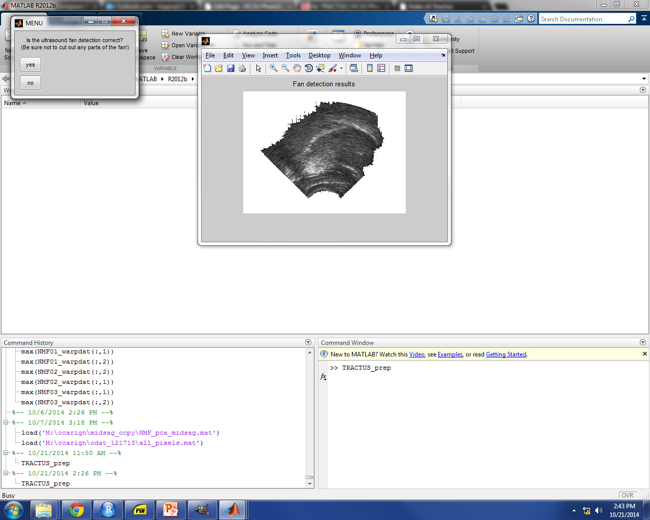
If the threshold is set too low, the automatic detection won’t be strong enough, and image area outside the fan border will be included (not good!). An example is shown in the image below for 4% threshold. In this case, you should select “no” and try a different threshold value.

If the threshold is set too high, the automatic detection will be too strong, and image area inside the fan border will be excluded (not good, either!). An example is shown in the image below for 20% threshold. In this case, you should select “no” and try a different threshold value.
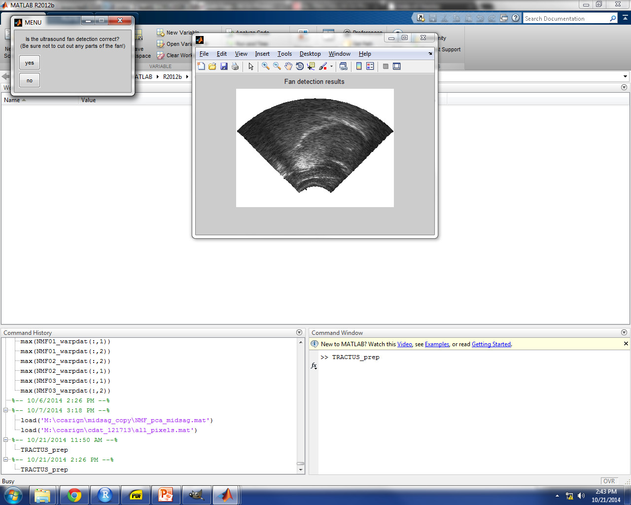
The correct threshold value for the image set should approximate the border of the ultrasound fan mask as closely as possible. An example is shown in the image below for 9% threshold, which provided a good approximation of the fan border for these images. Once you achieve the desired fan detection, select “yes” to continue.
FILTER PARAMETER SELECTION
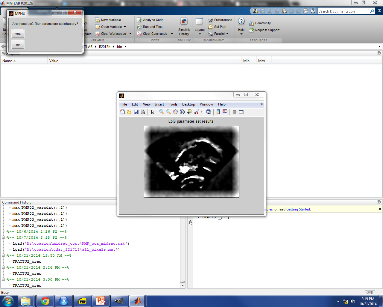
After fan detection, the next prompt will ask you to provide two parameters for image filtering, horizontal size (hsize) and sigma. A number of filters are applied to images, but these two parameters are used in the application of Laplacian of Gaussian filtering, since this is the filtering step which will impact the image contrast. 50 and 0.4 are suggested as default values to get you started. An image is selected from the middle of the data set, which will show you how the parameter values will affect the final filtered images. The goal at this step is to strike a balance between highlighting the tongue contour and minimizing image noise which is not associated with the tongue contour. Achieving this balance will take trial and error, as each ultrasound image set is unique. An example is shown in the image below for hsize 52 and sigma 0.4, which proved to be good parameter values for this particular image.
ROI (REGION OF INTEREST) SELECTION
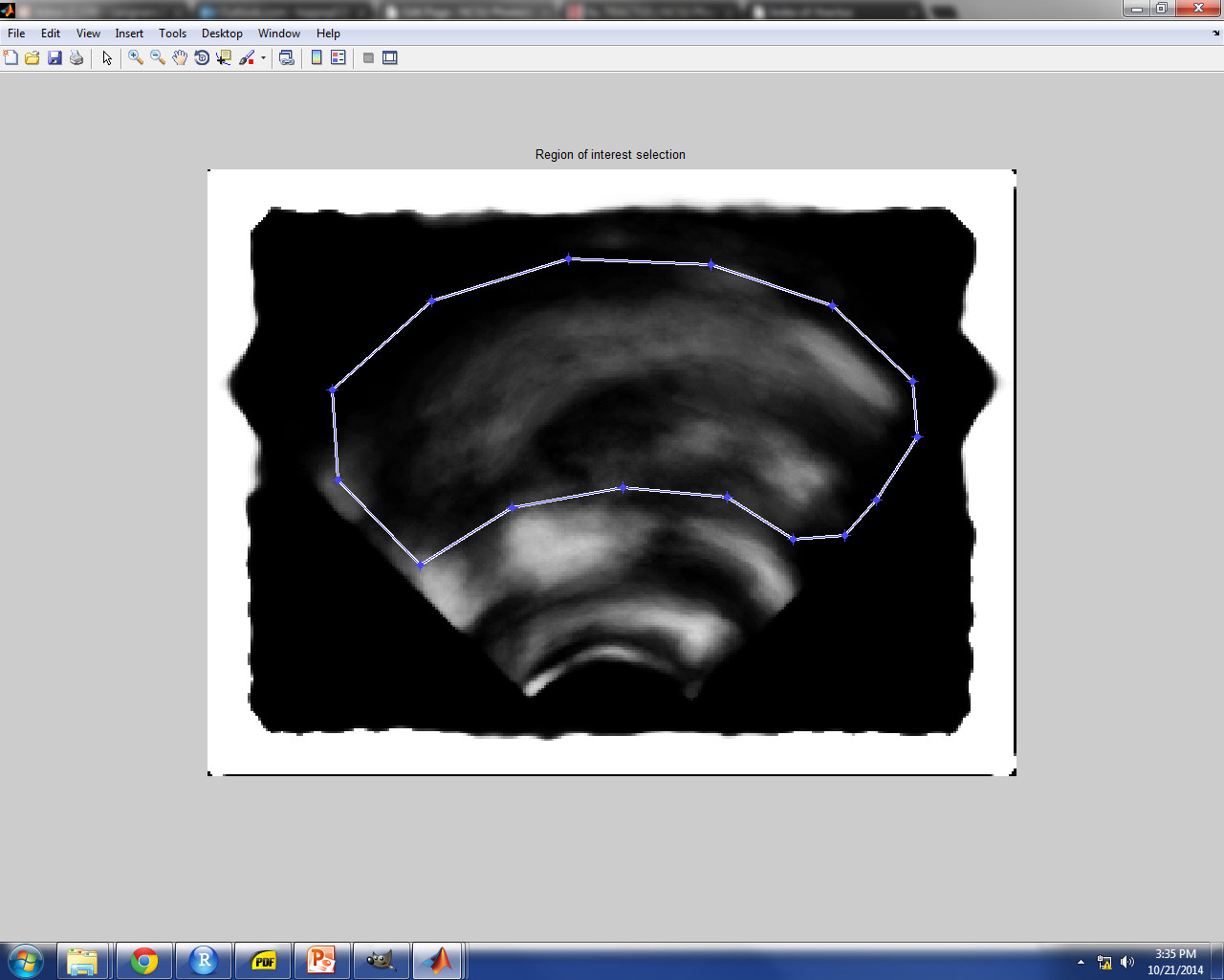
After a (possibly long) wait, you will be instructed to create a polygonal region of interest (ROI). It is up to your discretion as to how much or how little of the image area should be included in the analysis, but be aware that the size of the ROI will have a significant impact on the run time of the TRACTUS analysis. The ultrasound image which appears as a guide to assist in ROI selection is a composite image which represents an average of an evenly distributed 5% of the entire image set. As such, this image helps you to visualize where the tongue contour moves throughout the image set, and you can make your ROI selection according to this movement.
To select the ROI polygon, simply click points along the bounds of the desired area using the cross-hairs as a guide. To make the final point and close the polygon, click on the first point that you started with. Once the polygon is closed, you can adjust each of the points individually before finalizing the ROI. Once you are satisfied with the location of the ROI points, finalize the ROI by either double-clicking inside the polygon or right-clicking inside the polygon and selecting “Create Mask”. Another image will appear with a polygonal mask applied, where the image outside the ROI is blacked out. You must confirm whether the selection is correct. If it is not correct, select “no” and try again. If it is correct, select “yes” to finish. An example is given below of a polygonal ROI which includes movement of the tongue surface, but excludes image variance due to intrinsic lingual muscle movement.
At this point, the preparation is finished. You should verify that the prep file (“X_prep”, where X is the speaker name) has been saved in the results directory. This file is needed for the TRACTUS analysis.
TRACTUS Ultrasound Data Analysis
Once you have completed the preparation, the next step is to run the ‘TRACTUS.m’ function simply by typing ‘TRACTUS’ into the MATLAB Command Window and pressing Enter. A prompt will appear, asking you to select the proprietary file which was created and saved by the ‘TRACTUS_prep.m’ function (i.e. “X_prep”, where X is the speaker name). Once you select the preparation file, the following prompt will appear:
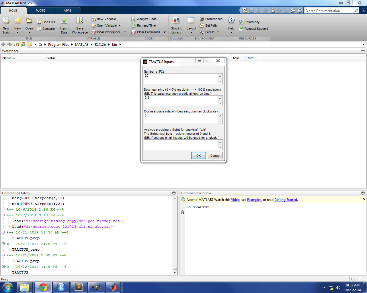
This prompt will ask you to provide four inputs:
- Number of PCs: the number of PCs that you wish to retain from the principle component analysis. This will determine the number of PC scores and PC heatmaps which are saved in the results directory. You may use as many or as few PCs as you wish, although a default of 20 is provided to get you started. It is recommended that you run TRACTUS once in order to determine the cumulative percentages of variance explained by successive PCs, and then a second time, retaining enough PCs to account for a large percentage of the variance. A rule of thumb is to retain as many PCs as account for roughly 80% of the total variance. The output file which provides these cumulative percentages is explained further on.
- Downsampling: the scale of image resolution to use in the analysis. Since downsampling the images before analysis not only reduces data dimensionality, but also processing load, this parameter may greatly affect the run time. The value for this parameter must be between 0 and 1, where 0 denotes 0% of the image resolution and 1 denotes 100% of the image resolution. A suggested value of 0.3 is provided as a default, which means that the images are downsampled to 30% of their original resolution. Downsampling is performed by binning adjacent pixels via bicubic interpolation.
- Occlusal plane rotation: if you know the angle of the bite/occlusal plane for your speaker, you have the option of rotating the images and resulting PC heatmaps to be parallel to this plane. This value is the number of counter-clockwise degrees you wish to rotate the image. A negative value can be used for clockwise rotation, if desired. A default value of 0 is provided; if this default value is used, the images will not be rotated.
- Filelist (y/n): if you want to perform analysis on only a subset of the images in your data set, you have the option to inform TRACTUS which images to include and which to ignore. For example, if you want the PCA model to only account for variance related to speech, a file list can be used to include only images related to speech events. If you want to use a file list, put ‘y’. You will be instructed to select the file list after clicking ‘OK’. The file list must be a text file (*.txt) which contains a single column vector of 0 and 1 values. The number of rows in the vector must match the total number of images in your data set. For each row in the column, 1 denotes an image which is to be included in the analysis and 0 denotes an image which is not to be included. If you do not want to use a file list, put ‘n’; in this case, all images in the data set will be used in the TRACTUS analysis.
After supplying the inputs for the TRACTUS analysis, click ‘OK’. A window will appear with an approximation of the time it will take for the analysis to be completed. Keep in mind that this is only an approximation: it is not intended to be exact. This approximation is based on the number of images, the size of the ROI, and the downsampling factor used. For the recommended 30% downsampling factor used on the images demonstrated here, TRACTUS can analyze roughly 6.5 images per second… that’s nearly 25,000 images per hour. In other words, if your ultrasound system records at 30 fps, TRACTUS can perform analysis on every frame in 10 minutes of ultrasound video in only 45 minutes… so go grab some lunch while you let TRACTUS do the hard work for you!
TRACTUS results
Once the analysis has been completed, the following results files will be available in the user-specified results directory:
*_filenames.txt: Contains the file names for each image used in the analysis, in linear order.
*_misc.txt: A log which contains the values of several variables which were used in the analysis.
*_pc_heatmaps.txt: Contains the heatmaps for each PC retained in the analysis. These heatmaps can be viewed by using the ‘pc_heatmap_plot.m’ function (explained here).
*_pc_scores.txt: Contains PC scores for each ultrasound frame. Rows are PC scores for each frame, and columns 1 to n are the scores for n PCs used in analysis.
*_res_heatmaps.txt: Contains heatmaps constructed from the residuals of the PCA model.
*_var_explained.txt: Contains a single column of combined percentages of variance explained by each PC, where row 1 is the percentage of variance explained by PC1, row 2 is the percentage of variance explained by PC1 + PC2, etc.
*_vecs.bmp: A bitmap image file which contains the vector matrix used in the PCA analysis.
working with TRACTUS Data
Viewing PC heatmaps
The heatmaps associated with each PC can be viewed by using the ‘pc_heatmap_plot.m’ function (requires the ‘scaled_heatmap.m’ function). Once the location of these functions has been added to MATAB’s path, they are ready for use.
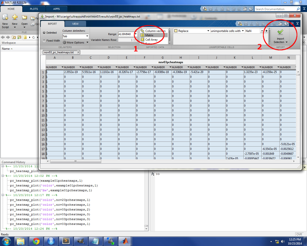
The first step is to import the heatmap file from you results directory. To do so, simply drag the *_pc_heatmaps.txt file from the results directory and drop it directly in the MATLAB Workspace. An import window will appear to ask you how you want to import the data. Choose “Matrix”, then click “Import Selection”. See the image below for an example. If you get an error when you click “Import Selection”, the data might not have loaded completely into MATLAB’s memory: try clicking “Import Selection” a second time to resolve this issue.
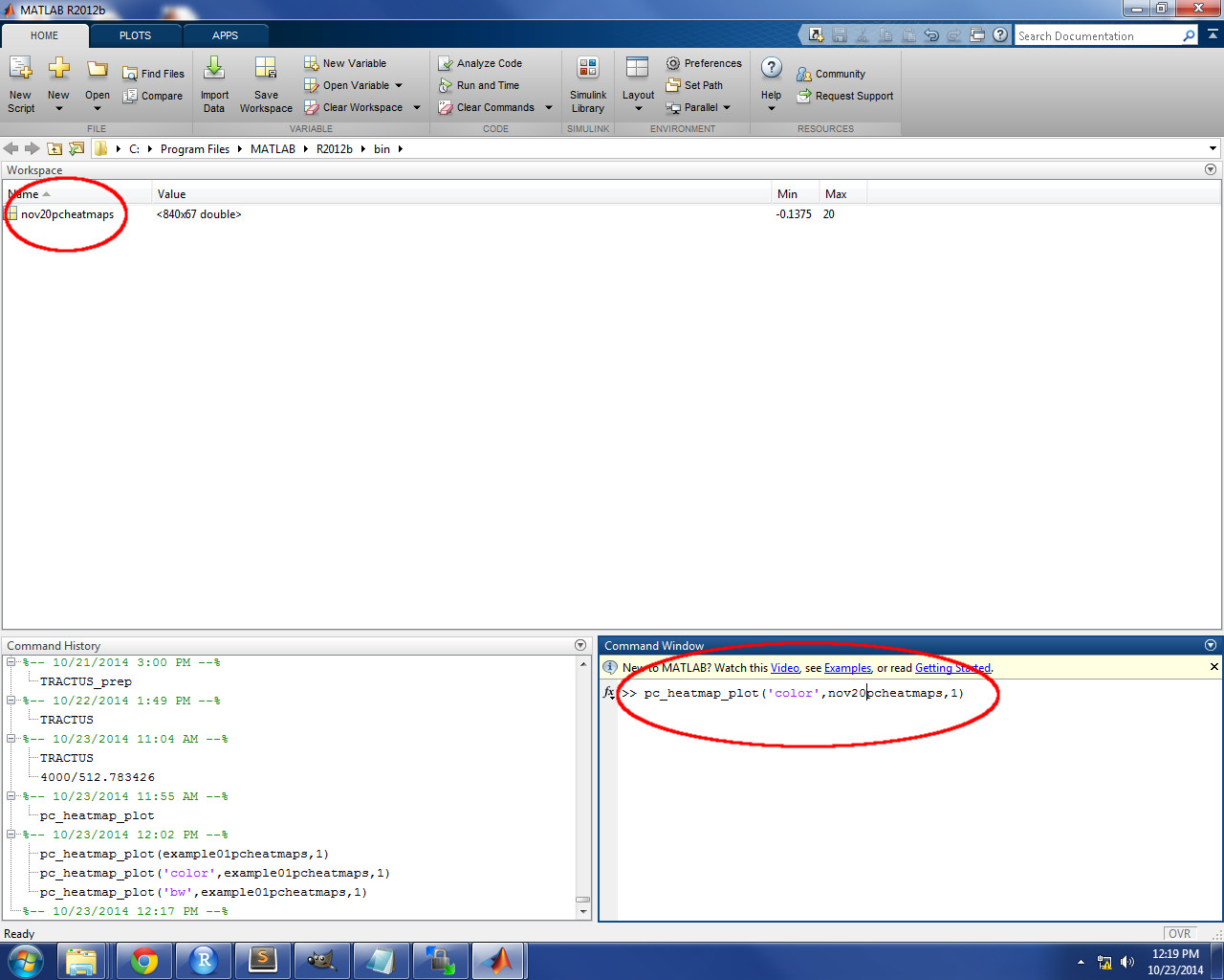
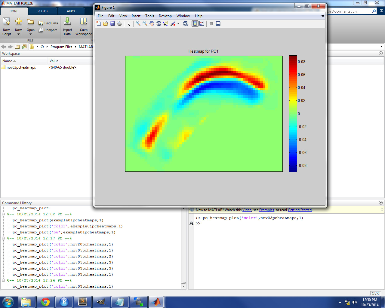
Once the heatmap file has been imported to the Workspace, call the pc_heatmap_plot function by typing ‘pc_heatmap_plot(type, pc_heatmaps, my_pc)’ into the Command Window, replacing ‘type’ with either ‘color’ or ‘bw’ (must be in single quotes), ‘pc_heatmaps’ with the exact name of the file as it appears in the Workspace (must not be in single quotes), and ‘my_pc’ with the PC number for which you wish to plot the PC loading heatmap. See the image below for an example.
When you run the function by hitting the Enter key, a plot will appear with a heatmap which displays the loadings (i.e. correlation coefficients) for the given PC, mapped onto their original spatial location in the image area. The PC loading heatmaps can be plotted in color by using ‘color’ as the input for ‘type’. In a color heatmap, pixels near the red end of the spectrum denote strong positive loadings (i.e. strong positive correlation with the PC) and pixels near the blue end of the spectrum denote strong negative loadings (i.e. strong negative correlation with the PC). In the image below, a color heatmap is displayed for PC1 loadings for an example speaker. For this speaker, individual ultrasound images which have a high positive score for PC1 will have a tongue shape similar to the red in the heatmap (i.e. the tongue body will be raised).
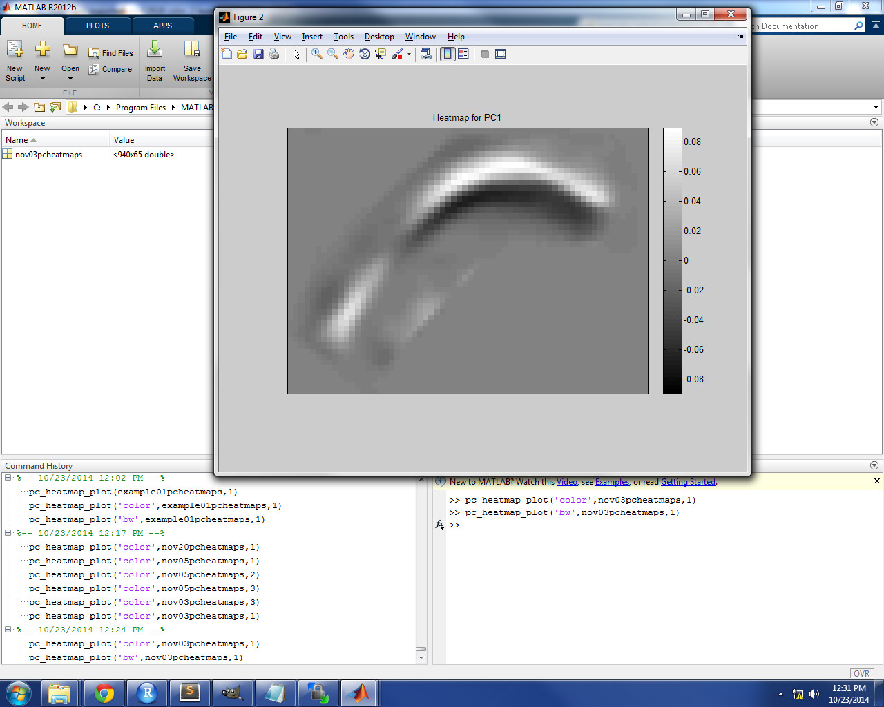
The PC loading heatmaps can also be plotted in grayscale by using ‘bw’ as the input for ‘type’. This is useful, for example, in journal articles which do not allow color images. In a grayscale heatmap, pixels near the white end of the spectrum denote strong positive loadings (i.e. strong positive correlation with the PC) and pixels near the black end of the spectrum denote strong negative loadings (i.e. strong negative correlation with the PC). In the image below, a grayscale heatmap is displayed for PC1 loadings for an example speaker.
Working with TRACTUS data
One of the advantages of using TRACTUS for ultrasound image analysis of speech is the ability to derive linguistically meaningful signals from PC score vectors. For example, the scores from the first 20 PCs can be retained as inputs to a linear discriminant analysis (LDA) model with classes based on groupings such as consonant place of articulation or peripheral location along some dimension of the traditional vowel quadrilateral (e.g., high-low vowels, front-back vowels).
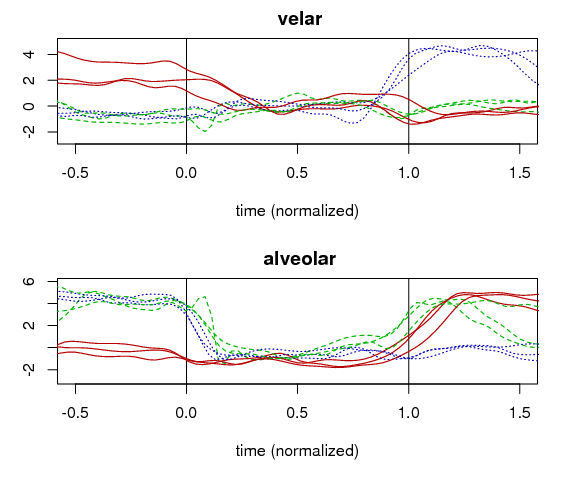
In the example shown below, two LDA models were created: one based on velar consonants [k g ŋ] in the data set vs. everything else, and another based on alveolar consonants [t d n s z] vs. everything else. The segmentation is based on the acoustic signal, and the classifier in the LDA model is based on the PC scores. The LDA class scores of the image set, when plotted sequentially as a temporal vector, generate a time-varying representation of the degree to which the imaged vocal tract matches the categories used to construct the LDA model. In this image, the velar and alveolar articulatory signals are plotted for multiple productions of the words ‘gas’ (red/solid line), ‘sad’ (green/dashed line), and ‘sag’ (blue/dotted line). For example, the alveolar signal in the image starts high for [s] in ‘sad’, lowers for [æ], rises in anticipation for the coda [d], and reaches a peak immediately following the vowel offset. The temporal resolution of this articulatory signal is equal to that of the ultrasound machine used (e.g., 60 Hz for the Terason t3000, used to record the data presented here).
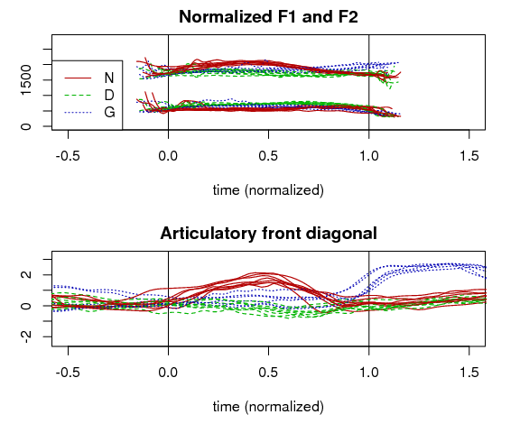
Another example of how to transform the PC scores is to identify the linear combination of articulatory PCs that best matches an acoustic dimension. For example, American English /æ/ tensing operates along the front diagonal of the vowel space (along a line approximating the axis between [a] and [i], quantified as Z2-Z1 (normalized F2 – normalized F1). In the image below, a linear regression was performed with dependent variable Z2-Z1 and independent variables PCs 1-20. Data was every frame during a vowel lying along the front diagonal [a æ ɛ e ɪ i]. The linear regression model was used to transform the articulatory data to match this “articulatory diagonal” for every frame at the original frame rate. The bottom subfigure in the image shows the front diagonal articulatory signals for several repetitions of English words with /æ/ before /n/ and /g/, where there is tensing for this speaker, and /d/ where there is no tensing. This dynamic representation of tongue posture shows that: 1) tensing is greater before /n/ than before /g/, and 2) tensing has a falling tongue trajectory before /n/ and a rising tongue trajectory before /g/.
Citing/referencing TRACTUS

The TRACTUS functions are freely available for non-commercial use
with the condition that the author and website are properly
acknowledged:

Carignan, C. (2014). TRACTUS (Temporally Resolved Articulatory
Configuration Tracking of UltraSound) software suite.
URL: http://phon.chass.ncsu.edu/tractus.
Back: Preparing and Analyzing Ultrasound and Video Data
Return to Ultrasound and Video