
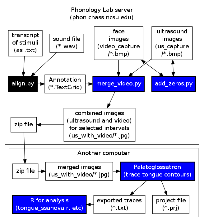
This page includes retrieving the data from the server, preparing TextGrids and merging data, and how to use different methods of analysis, including palatoglossatron (Windows or Mac).
See also: Other Methods of Ultrasound Analysis is a page that covers
alternative methods for ultrasound data analysis. It includes
information on Principal Component Analysis (PCA), done in MATLAB,
and Temporally Resolved Articulatory Configuration Tracking of
UltraSound (TRACTUS).
Preparing your Data for Analysis
Once you have collected the data from the ultrasound recording session, there are several options when it comes time to process the images in preparation for subsequent analysis as well as the type of analysis itself. This section will offer information on how to:
- Synchronize your Data
- Prepare for Contour Analysis
Syncrhonizing your data
This step involves uploading your files to the server and preparing them using the add_zeros.py script. If you are not using merge_video.py, there are also instructions for converting the .bmp files to .jpgs and preparing them for download. The following instructions are for synchronization.
For these instructions, we are assuming your file is called mydata.zip. If your file is named something else, replace the “mydata” with the name of your file. Some useful unix/linux commands are:
- mv [path to file] [path to new location of file] = move
- cp [path to file] [path to location of copy] = copy
- ls = list directory
- cd [path to directory] = change directory
- unzip [zipfilename] = unzip a zip file
- zip [zipfilename] [filestozip] = make a zip file
- python [path to script] = run a python script
- vi = open a text editor
- man [command] = show the documentation (manual) for any command
- To unzip your file:
unzip mydata.zip
(this may take a while)
- The script expects your audio file to be in audio_capture and the TextGrid file to be in the main mydata directory (created when you unzip the file). The following command will move the TextGrid where it needs to be, as long as you uploaded your TextGrid file to your home directory. (~/ is equivalent to typing the path to your home directory):
mv ~/mydata.TextGrid /phon/ENG536/mydata/
- Change to the mydata directory and get a directory listing:
cd /phon/ENG536/mydata
ls
You should see the three subdirectories, the audio file, the textgrid file, and the report file.
- List the ultrasound image files:
ls us_capture
- You should see that the time stamps are not all the same number of digits. To fix that, we’ll need to run a python script that is located in the /phon/scripts directory:
python /phon/scripts/add_zeros.py us_capture/
python /phon/scripts/add_zeros.py video_capture/
IF YOU WOULD LIKE TO DOWNOAD JPG VERSIONS OF YOUR IMAGES: At this point your images can be analyzed by tracing the contours or by doing a principal component analysis, as described in the next two sections. If for any reason you want to download your images at this point (e.g., if you don’t plan to use merge_video.py) and want to convert the bitmap images to jpgs for their smaller file size and/or delete the .loc files, run one or both of these lines in the terminal:
mogrify -format jpg -quality 60 yourpath/us_capture/*.bmp
rm -f yourpath/us_capture/*.loc
To zip up the files along with a text file containing a list of their names:
ls yourpath/us_capture | grep 'jpg' > list_of_your_files.txt
zip -qj yourpath/your_jpgs yourpath/us_capture/*.jpg
Preparing for Contour Analysis
This section instructs you on how to align your ultrasound images with the audio recording you made in preparation for using merge_video.py. Even if you do not have camera images, this step is useful for associating your segmentation with the ultrasound images. The script also converts your images to smaller .jpg files.
USING MERGE_VIDEO.PY
NOTE: These instructions assume you used Ultraspeech 1.3, recording audio and ultrasound (and possibly video) together. Scroll to the bottom of this page for further instructions relevant to Ultraspeech 1.2
Make a TextGrid annotation of your wav file either manually in Praat or automatically using a forced aligner. You will need two interval tiers, called “phone” and “word”. If your recording includes palate images (the mouthful of water) you should add a “palate” interval on the phone tier. If your recording includes occlusal plane images (the tongue depressor between the teeth) you should add an “occlusal” interval on the phone tier. Ultraspeech 1.3 currently makes only 32-bit wav files, but many of the aligners we use expect 16-bit wav files. It’s easy to make a 16-bit copy and use it for forced alignment:
sox audio_capture/mydata.wav -b 16 audio_capture/mydata16.wav
python /phon/p2fa/align.py audio_capture/mydata16.wav mydata.txt mydata.TextGrid
The images created during the word intervals you segment are the ones that will be processed (if you created the TextGrid somewhere else, upload it to the server using scp or winSCP).
IF YOU WOULD LIKE TO MAKE A VIDEO CLIP: At any time, you can make a video clip of your ultrasound or video data, using a command like this (replacing the start and end times with times you select from your textgrid):
python /phon/scripts/makeclip.py --wavpath audio_capture/mydata.wav --start 62.533 --end 64.641 --output mydata_token1
Prepare your lip images (if applicable). If you have lip images, the lips themselves probably only occupy a small part of the middle of the frame. We need to crop the images to make them easier to analyze. First let’s sample the video images to decide where to crop:
python /phon/scripts/bmpsmpl.py --output mydata
Looking at mydata_summary.bmp (created by the script) will help you choose a rectangular mask. Each block is 80×80 pixels. The four numbers you need to come up with are the width and height of the box that will enclose the lips and the x and y coordinates (starting at the top-left) for the top-left corner of the box. Enter these as the crop argument ([width]x[height]+[top-left-x]+[top-left-y]) as in this example:
python /phon/scripts/makepng.py --textgrid mydata.TextGrid --crop 400x240+80+80
This step also converts the bmp images to the more efficient png format and exclude frames that aren’t near speech intervals. You can do this even if you don’t have video images. Just leave out the crop argument. This saves a lot of disk space, because the png images are smaller than bmp images, and you can delete the ones that aren’t near speech intervals:
python /phon/scripts/makepng.py --textgrid mydata.TextGrid
makepng.py will create two scripts that do the actual conversion: a test script (to see if you like your lip image cropping) and a convert script (to convert all the images).
./mydata_test
Now you can look at images in video_png and/or us_png and make sure you’re happy. If you want to change the lip image cropping, re-run makepng with different numbers.
nohup ./mydata_convert &
We are using nohup to run the convert script in the background, because it might take a long time. To check whether the convert script is done, use these five commands. This means “how many images am I trying to convert?”:
grep -c png mydata_convert
These four commands mean “how many images have I created in the four directories that might hold images?”:
ls palate/ | grep -c png
ls occlusal/ | grep -c png
ls us_png/ | grep -c png
ls video_png/ | grep -c png
You can keep pasting these commands until the numbers add up to the number you got above. That means all the images that were supposed to be created have been created. If you don’t have intervals in your textgrid’s phone tier labeled “palate” or “occlusal”, these directories should be empty.
While logged into the server (in the directory where your files are), copy the configuration file we’ll need for the next script (./ is equivalent to typing the path to the current directory):
cp /phon/scripts/merge_video_settings.txt ./
The settings file contains many different parameters that are important for the video merging process. Most settings can stay the same, but at the very least you will need to edit it to give it the correct name of your textgrid, and if you made a direct-to-disk recording, you will need to enter the video time offset. You can download the settings file, edit it, and then upload it, or learn how to use the text editor vim:
vim merge_video_settings.txt
You will see the top of the text file. Use the arrow keys to get to the line that starts with textgrid_fn;. To insert text, first press the i key. Then change the rest that line to the correct TextGrid file name. The other things you are likely to want to change here are:
- list specific phones in the seg_label_equals line
- If you ran makepng.py, scroll down to FILE LOCATIONS and change us_capture and video_capture to us_png and video_png. This will process the new png images instead of the original bmp images.
- If you want to extract only the middle frame of each interval, scroll down a little further and change middle_only;0 to middle_only;1
- If you want to make two versions of the output (such as one with middle frames and one with all frames, you can change us_with_video (under FILE LOCATIONS) to us_with_video2
When you are done editing the file in vim, first press escape, then colon, then enter in wq to write, then quit.
Now run the merge_video script to select and merge the video frames:
python /phon/scripts/merge_video.py
This may take a long time, depending on how much you extract.
By default, the merged images will appear in a folder called us_with_video. To download the images as a file called myimages.zip, zip them first:
zip myimages us_with_video/*
Next, use scp or WinSCP to download the zip file. If you use scp, this is the command to use:
scp unityID@phon.chass.ncsu.edu:/phon/ENG536/mydata/myimages.zip ./
That will probably put the zip file in your home directory on your computer, but you can change ./ to a different location if you prefer.
Unzip the zip file and look at the merged images. If they look good, you can proceed to analysis. Otherwise, you may want to change settings in merge_video_settings.txt and run merge_video.py again.
VERIFYING SYNCHRONIZATION
As far as we know, the time stamp in the ultrasound and video images can be trusted. This means that once we determine the offset between the time in the time stamp for each type of video and the time in the audio, we can convert any audio time into a video or ultrasound time.
If you need to check synchronization and you don’t have the 15-second wav file for some reason, you can find the offset by comparing audio and images, it is necessary to have an event that starts abruptly and can be observed on more than one channel, for example:
- Audio, video, and ultrasound:
- squirting gel onto the transducer using a hammer
- audibly tapping a probe with a glob of gel on it against a surface
- Audio and video:
- clacking a Hollywood-style clacker
- a hand clap
- Audio and ultrasound:
- the release of a lingual stop
- Video and ultrasound:
- the release of a labial stop
Analyzing your Data
The next steps are dependent on how you have decided to tackle the analysis of the data obtained from your ultrasound recording. The following information is for CONTOUR ANALYSIS, which is tracing either the tongue or the lips, using the Palatoglossotron and SS ANOVA. It includes information on:
- Tracing with Palatoglossotron
- Using SS Anova to Compare Contours
Tracing with Palatoglossotron
We typically use Palatoglossatron to trace the tongue and lips. Refer to the Palatoglossatron manual for instructions on using Palatoglossatron to analyze ultrasound images. It is also possible to use EdgeTrak or the other programs that have been written for analyzing this type of data.
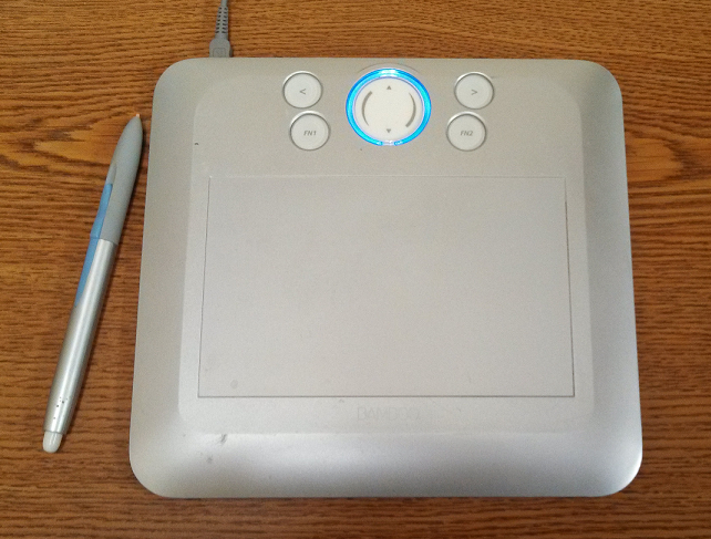
Figure 1. Tablet for tracing ultrasound images in Palatoglossotron.
Palatoglossotron is a Windows application that is used for processing ultrasound data that we gather in the Phonology Lab. An implementation of Palatron and Glossotron algorithms, it is designed to allow the user to easily and flexibly make traces of tongue and palate contours.
Palatoglossatron will not currently run in Linux on lab computers, but should run on any of the Windows computers in the Phonology Lab or the Linguistics Lab, or your own computer.
INSTALLATION
Download Palatoglossatron from here. You will need to unzip it and then rename Glossatron.ex_ to Glossatron.exe.
In Windows, it should just run as a normal program. Don’t move any of the files from where they are in the PG folder. Run Glossatron.exe. You can make a shortcut to Glossatron.exe on your desktop but don’t move the file.
In Mac OS or Linux, you will need to use WINE (a program that helps you run Windows programs in other operating systems). Here are instructions for installing WINE on a Mac. Then you should be able to run Palatoglossatron by typing this in a terminal (and substituting your actual path to Glossatron.exe, wherever you downloaded it to) or by following the opening instructions in the WINE instructions page:
wine /pathtopalatoglossatron/Glossatron.exe
As said in the Palatoglossotron manual, the only files that are needed to run are the .exe file and the .bin files. All others are unnecessary, but don’t delete them. For Windows users, you will have to make sure to change the .ex_ extension to .exe by renaming the file before being able to run the application.
STARTING A NEW PROJECT
Click on “new project” under File or use the command Ctrl + N (Windows). Browse to the file location and name your new project. Remember, typically each recording session or participant will take its own individual project. You also have to add the .prj extension to the project name at this time. Ordinarily we group palate images with tongue images, so you won’t need to add any palate files in the top box. For tongue images, click “add directory” and find the location of your images. Leave “dummy filename” alone.
Before clicking “OK”, you can click “Sort filenames…”, and you can change the delimiter (at the bottom) to .jpg (instead of an underscore). This will help later in the export process.
TRACING THE IMAGES
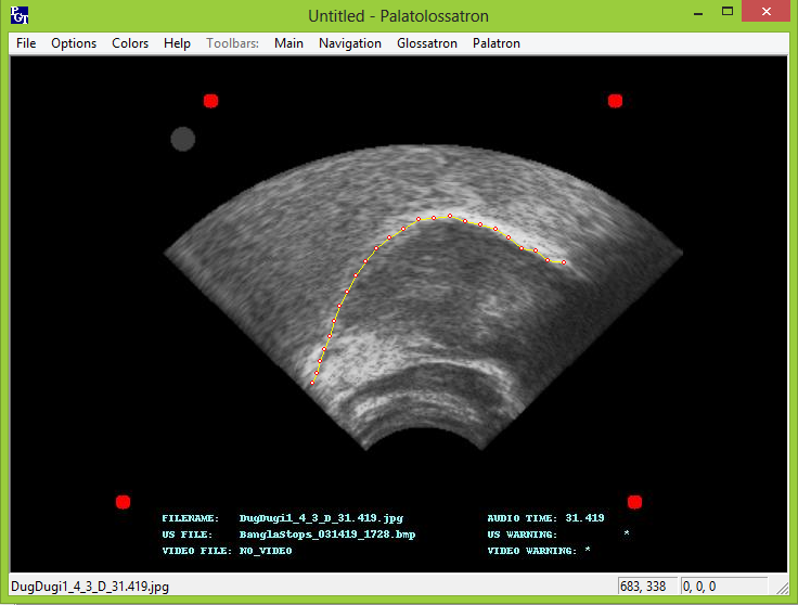
Figure 2. The Palatoglossotron user interface
Generally, you will find it most useful to read through the Palatoglossotron manual yourself in order to familiarize yourself with the tongue tracing process. Also refer to Stone 2005 for a thorough introduction to analyzing tongue contours from ultrasound images. However, there are a few important things to point out. The surface of the tongue is just below the bright white line; this is where the tongue meets the air and the ultrasound beams scatter. After tracing a project, it is advisable to clear orphans from all traces. These are stray, disconnected points. Be aware that erroneous traces of 2 or more points will not be erased by this process.
For lip data, you must press 1, 2, 3, and 4 to mark four locations on the lips that you can track throughout the duration of the phone. It is crucial to attempt to mark the same location on the lip with the same number every time, or your data will not be useful.
EXPORTING THE DATA
Before you export the data, you should go to the Options…Project options… menu and change the delimiter to .jpg (instead of an underscore). This will ensure that all the information from the image names gets exported.
When you are ready to export data from your tracings, you have the option to select from several formats. The one that is most useful for making smoothing-spline ANOVA comparisons is the R/SSANOVA format. Select this option from the Format menu, name your Output Filename, and select the relevant images you would like to export. Most likely you will want to check “Export data from tongue images” and “Raw tongue trace” and leave everything else unchecked. Your output file will appear in the same location as your .prj file and will include X and Y coordinates with values in pixels, as well as word label and token counts. It’s likely that you will want to transform your data from this point, but this is the minimally required format for performing an SSANOVA analysis in R.
Once images are traced, it is possible to make specific measurements of the traces (e.g., the highest point of the tongue body or the coordinates of points in a particular radius. Broad comparisons of sets of tongue shapes can be made using SSANOVA.
Should you wish to export lip data, you should instead export with the tab delimited format, check the box to export dot positions, and leave everything else unchecked. Your output file will appear in the same location as your .prj file, and will contain plenty of values of -1; the important values to look for are Aux1.x, Aux1.y, Aux2.x, etc. through Aux4.y. These will be the X and Y coordinates of your four dots used to trace the lips, in pixels..
Using ss ANOVA to compare contours (SMOOTHING-SPLINE COMPARISONS)
tongue_ssanova.r is a set of R functions for making Smoothing-Spline ANOVA comparisons using the gss package. If you don’t have the gss package already you can install it by typing install.packages(‘gss’) or by using menus, depending on your operating system. The gss package contains many functions that you can use directly, and you can find the manual here. tongue_ssanova.r is meant specifically for working with tongue traces.
If you load a data file in the R/SSANOVA format into R as data and you have tongue_ssanova.r saved locally, you can use commands like this to generate SSANOVA comparisons, which will compare ALL your data with word as the factor (probably not what you want):
source('tongue_ssanova.r')
data <- read.csv('myPGexport.txt', sep='\t', h=T)
ss <- polar.ssanova(data)
The source function needs to find tongue_ssanova.r using the correct path; either change your working directory in R or specify the path to its location on you computer. The functions in tongue_ssanova.r expect your data frame to have columns X and Y, and it will assume your factor is in a column labeled word. You can use the separate_token() function to separate the token column into meaningful information like repetition, phone, and frame time:
data <- separate_token(data)
If this command does not work, go back and change your delimiter in palatoglossatron from ‘_’ to ‘.png’ or ‘.jpg’.
These are standard in the R/SSANOVA format, but if you can specify other columns like this:
ss <- polar.ssanova(data, 'phone')
You will probably want to subset your data and reduce the factor levels before making comparisons. If for example, you only wanted to look at data for the phones ‘a’ and ‘i’, you might use these commands:
subdata <- subset(data, phone%in%c('a','i'))
subdata$phone <- factor(subdata$phone)
ss <- polar.ssanova(subdata, 'phone')
Plotting directly to file is highly recommended as a way to maintain control over the size and uniformity of your plots (using the height and width arguments), and to put multiple plots in a single pdf file:
cairo_pdf("ssanova_by_speaker.pdf", height=4.5, width=5, onefile=T)
   ss <- polar.ssanova(data1, main='speaker 1')
   ss <- polar.ssanova(data2, main='speaker 2')
   ss <- polar.ssanova(data3, main='speaker 3')
dev.off()
You can also use commands such as png() and jpeg() if you need bitmap images instead of pdfs. The disadvantages of these formats are that they look bad when they are enlarged (because they are made of pixels instead of vectors), and they don’t support multiple pages. pdf and eps are good formats for making graphics files to insert into LaTeX documents, but they may be harder to insert into Word documents.
PLOTTING RAW DATA
It is often useful to plot the tokens directly, to see how they are distributed and if there are any apparent outliers. This can be done using the following function:
show.traces(data)
To highlight the traces for the category ‘PIN’, use this:
show.traces(data, c('PIN'))
To show only the traces for the category ‘PIN’, use this:
show.traces(data, to.plot=c('PIN'))
The polar.ssanova() function converts tongue traces into polar coordinates in order to make comparisons that are roughly perpendicular to the tongue surface, and then plots the results in the original Cartesian coordinate system. This is probably the most appropriate way to deal with tongue trace data in most circumstances, because we are rarely interested in making comparisons that are perpendicular to the x-axis but arbitrarily oblique to the tongue surface.
FUNCTION PARAMETERS AND OTHER FUNCTIONS
polar.ssanova() and show.traces() might be the only functions you need to use, but you can call the other functions in tongue_ssanova.r directly, or directly use the gss functions. polar.ssanova() has some graphical parameters you can change. You can also modify plot.tongue.ss() (the function that does the actual plotting), or just take the data frame returned by polar.ssanova() and plot it using ggplot or anything else. The data frame contains the factor used to categorize the traces (probably word), the coordinates of the splines (X and ss.Fit), and the coordinates of all the points in the upper and lower edges of the confidence intervals. [The bounds of the confidence intervals are equal to the fit line plus/minus 1.96 times the Standard Error in polar coordinates, but when they are returned to Cartesian coordinates they need to be treated as separate curves, because they aren’t strictly above and below the points in the fit line anymore.]
polar.ssanova() takes the following optional arguments:
- tongue.cat: the factor to use to categorize the tongues (defaults to ‘word’)
- scale: how much to scale the axis values (e.g. to convert from pixels to centimeters)
- origin.method: how to choose the origin for calculating polar coordinates
- debug: whether to generate the cartesian and non-transformed polar plots too
- plotting: whether to plot anything (or just return the result of the test)
- main: the main title for the plot
- CI.fill: whether to indicate confidence intervals with shading (like ggplot) or with dotted lines (like the earlier SSANOVA code). Defaults to FALSE (dotted lines)
show.traces() takes the following option arguments:
- data: your tongue tracings (minimally including columns X and Y and a column with a factor)
- to.highlight: a list of factor levels to plot while muting the other levels
- to.plot: a list of factor levels to plot, excluding the rest (defaults to all)
- tongue.cat: the factor to use to categorize the tongues (defaults to ‘word’)
- main: the main title for the plot
- overplot: whether to add the traces to an existing plot
The old instructions for making SSANOVA comparisons using the assist package can be found here.
LIP DATA FROM PALATOGLOSSATRON
If you traced lip data in Palatoglossatron, make a second export using tab-delimited format. Since you exported your tongue traces in SSANOVA-friendly format you can ignore everything in the export except filenames and columns labeled Aux1.x, Aux1.y, etc., which contain the x and y coordinates of the points you traced. After you open it in R you will need to use the separate_filename() function to get information from the filenames.
source('tongue_ssanova.r')
lipdata <- read.csv('myPGtabdelimitedexport.txt', sep='\t', h=T)
lipdata <- separate_filename(lipdata)
If you traced the upper lip as Aux1 and the lower lip as Aux2, a reasonable thing to do would be to plot their vertical distance:
lipdata$vert <- abs(lipdata$Aux1.y-lipdata$Aux2.y)
boxplot(vert ~ phone, lipdata)
Missing values are treated as -1, so this distance will be 0 for anything you didn’t actually trace. You may or may not want it to work that way.
See also: Other Methods of Ultrasound Analysis is a page that covers alternative methods for ultrasound data analysis. It includes information on Principal Component Analysis (PCA), done in MATLAB, and Temporally Resolved Articulatory Configuration Tracking of UltraSound (TRACTUS).
Back to In The Lab: Generating and Recording Ultrasound Images
Back to Main Page: Ultrasound and Video
or, if you were using Ultraspeech 1.2, continue below
Extra steps needed for Ultraspeech 1.2 recordings
If you made a direct-to-disk recording with Ultraspeech 1.2 or earlier, you will need to calculate the time offsets between the channels first. If you use Ultraspeech 1.3 made a RAM-to-disk recording, skip to step 1.To align your ultrasound and video images, determine the filename of the first image of each channel. The naming scheme for direct-to-disk ultrasound images is this:
[basename]_[ms from recording start]_[frame number in cine loop].bmp
but the naming scheme for direct-to-disk video images is this:
[basename]_[ms from boot up]_[frame number in recording].bmp
so the first ultrasound frame has the lowest number in the middle, and the first video frame has the lowest number at the end. Find them by typing these two commands in the directory where your files are:
ls video_capture/ | grep '_1.bmp'
ls us_capture/ | grep '_0000.*bmp'
These commands us “ls” to list all of the images images, but instead of showing them all to you, it pipes them to the program “grep”, which finds the filenames that match certain strings.
chass% ls video_capture/ | grep '_1.bmp'
myname_2393351_1.bmp
chass% ls us_capture/ | grep '_0000.*bmp'
myname_000000_18.bmp
myname_000004_19.bmp
myname_000007_28.bmp
myname_000008_20.bmp
myname_000009_21.bmp
...
There should only be one video file that has _1.bmp in its name (the first frame), and there should be a small number of ultrasound frames that have time stamps starting with four zeros (the first several). Since we know the first video frame is 2493351, we know that the video time stamps are 2493.351 seconds ahead of the ultrasound time stamps. This is the number we will need to put in merge_video_settings.txt.
To align your audio recording with your Ultraspeech recordings, the easiest technique is to use the 15-second recording made by Ultraspeech and crop the long wav file so that it starts at the same time as the images. If you started it after you started recording in Audacity, you just need to find the 15-second stretch of the long recording that matches to match up the files.
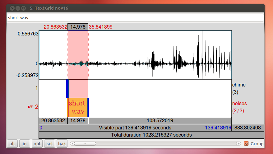
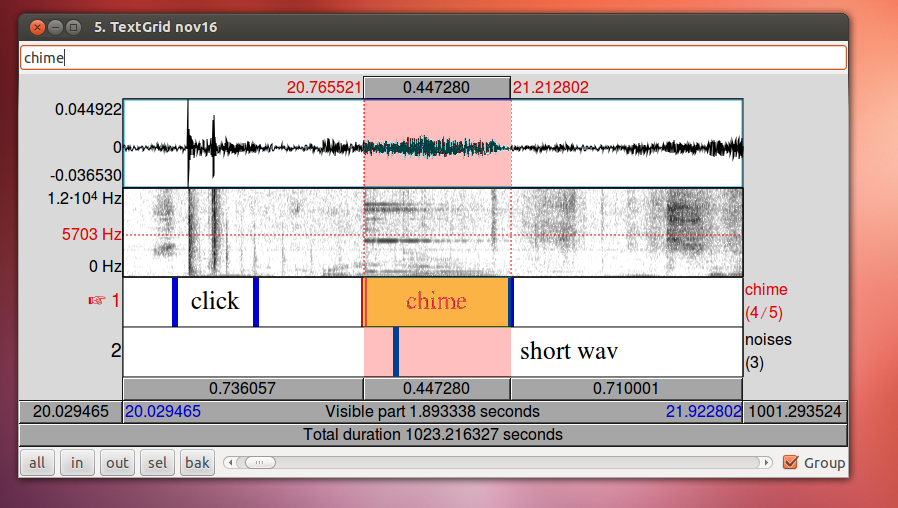
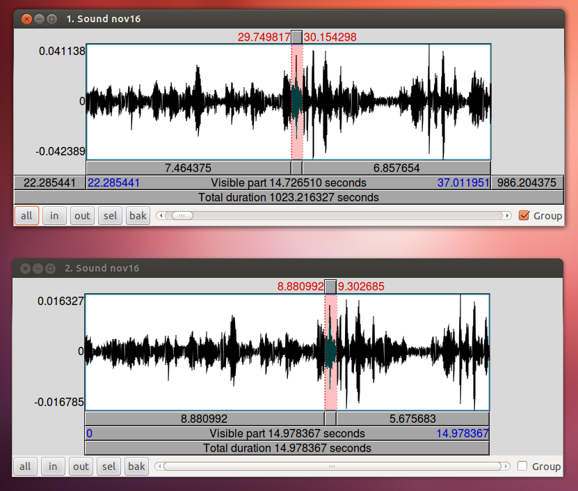
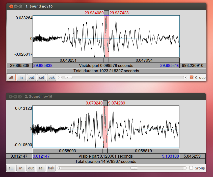
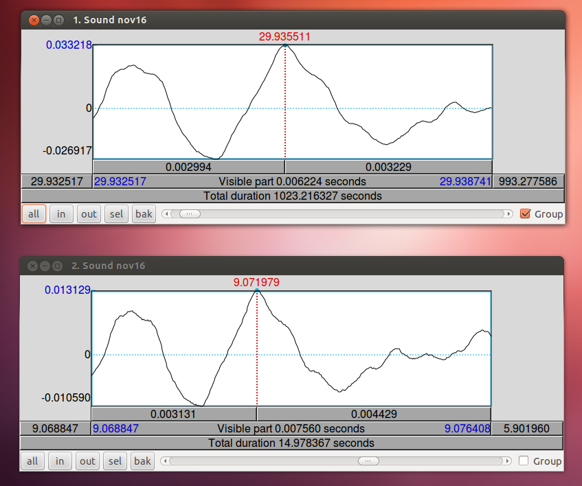
When you have zoomed in on the same peak in both wav files, subtract the difference in time. In this case, 29.9355 – 9.0720 = 20.8635. The long wav file started 20.8635 before Ultraspeech started recording. We need to crop off the first 20.8635 seconds of it. You can do this in Praat using Extract part… Afterward, you can check the alignment by combining it to stereo with the 15-second wav file. They should look identical. Upload your new cropped wav file to the server and use it to continue with your analysis.
When editing merge_video_settings.txt (above), you will need to do these things too: To set the video frame offset, find the line that starts with “default_video_offset;” and change the number 0 to time in seconds that you got from inspecting the frame filenames. In the example, the first video frame had time 2393351, so we need to enter 2393.351 here. Scroll down to see the other options available in the file. Some are not useful to you, and some may become very useful in the future. You will probably need to change video_x_offset in order to position the speaker’s mouth somewhere that it’s not obscured by the ultrasound image, but that will be easier to do after you have run the script once. When you are done inserting text, press the ESC key, followed : and x to exit vi and save the file.